Recent researches have leveraged Generative Adversarial Networks (GANs) for generating photo-realistic images and performing image manipulation. However, to perform such manipulation on real images requires understanding its corresponding latent code. This series intends to explain the concept of GAN Inversion [1], which aims to provide an intuitive understanding of the latent space by inverting an image into the latent space to obtain its latent code.

The series is structured into the following four parts:
- Part I — Introduction to GAN Inversion and its approaches.
- Part II, III & IV — GAN Inversion extensions, applications, and future work.
This post is the first part of a four-part series on GAN Inversion. It aims to provide a brief introduction to GANs [2] and their latent spaces, in addition to introducing the concept of GAN Inversion [1] and its approaches and shows a brief comparison with Variational Autoencoders.
This blog is inspired mainly by the GAN inversion survey by Bau et al. [1], while we also explore some of the newer extensions in the field. Let’s first dive into a brief introduction to GANs and their latent spaces.
1. Background
1.1 Generative Adversarial Networks
Generative adversarial networks (GANs) are deep learning-based generative models, referring to models aiming to generate new, synthetic data resembling the training data distribution. These differ from discriminative models intending to learn boundaries between classes in the data distribution. GANs were first proposed by Goodfellow et al. [2], and various models have been developed since then to synthesize high-quality image generation.
GANs comprise of two main components:
- Generator (G): aims to learn the real data distribution to generate data closer to the distribution and fool its adversary, the discriminator.
- Discriminator (D): aims to discriminate between real and generated images.
Goodfellow et al. [2] propose to train the generator and discriminator components together with opposing objective functions striving to defeat each other. The model converges when the generator successfully defeats the discriminator by generating data indistinguishable from real data. The objective function proposed is as follows:

where 𝔁 represents the data and 𝒛 represents a random noise vector. As can be seen, the discriminator maximizes the objective function while learning to perform the distinction, while the generator minimizes it by generating realistic data.
The network architecture can be seen in Fig. 1.

1.2 GAN latent space
During the training procedure, randomly selected points from the distribution are passed through the generator to generate synthesized images. The discriminator learns to differentiate between the real training dataset images and the synthesized images, labelled as real and fake respectively, as a classification approach.
The generator learns patterns in the distribution space, mapping a location in the space to specific characteristics in the generated image. This N-dimensional space with a GAN’s learned patterns is the GAN’s latent space, generally referred to as the Z space. The vectors in the latent space, including the random noise vectors mentioned earlier, are termed latent vectors. The latent space differs each time a GAN model is trained.
While we did not find much reasoning on why nearby points in the GAN distribution space have similar characteristics, the understanding is that it is to do with the internal mechanisms of GANs.
Recent researches have shown that well-trained GANs encode disentangled semantic information in their latent space. These researches do so by introducing spaces in addition to the Z latent vector space to better incorporate the style and semantic information within the space.
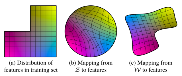
StyleGAN [4] introduced the W space in order to incorporate semantic information into the latent space. Fig. 2 illustrates this. For example, we have a dataset of human faces, which lacks images for some combination of features, e.g., long-haired males. In this case, (a) represents the distribution space for the combination of the features, e.g., masculinity and hair length. (b) represents the Z space, where the mapping becomes curved/entangled to ensure that the entire space incorporates valid feature combinations. This leads to these feature entanglement in the Z space. (c) represents the mapping of Z space to W space, introduced by Xia et al. [4] to obtain more disentangled features in the W space.
Other researches have proposed the W+ space [3], S space [5] for spatial disentanglement, and P space [6] for regularizing StyleGAN embeddings.
Many studies report disentanglement from a qualitative point of view. However, there still lacks a good evaluation metric for the perceptual quality of a generated image and its comparison with the expected outcome.
A well-trained GAN must be capable of generating realistic images as well as enabling image manipulation. It must also enable interpolation between the latent codes of two images to generate images with a smooth transition.
For instance, [3] defines the interpolation in the W+ space as follows:
where the step factor, λ, for interpolation is defined to be:
w₁ and w₂ are latent vectors for the two images to interpolate between, and w is the interpolated latent vector.
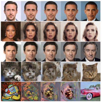
Fig. 3 shows linear latent space interpolation performed by Image2StyleGAN [3], trained on face images, in their W+ latent space. It can be seen that the GAN performs interpolation well on face images while failing to interpolate for non-face images realistically. This is due to the non-face images lying outside of the training data distribution.
It is also possible to apply specific changes to the image by modifying the latent codes in semantically meaningful directions. However, such manipulation requires a known latent vector for the corresponding image, hence is only directly applicable to images generated using the GAN. Performing such operations on real images requires their latent vector to be obtained, leading to research in the inversion of GANs.
This review aims to provide an overview of [1] and a detailed analysis of some GAN inversion researches. Hence, we won’t be going into a detailed overview of GANs. The remainder of this post focuses on GAN inversion and approaches. More information on GANs and their latent space can be found in [2].
2. GAN inversion and approaches
2.1 GAN inversion
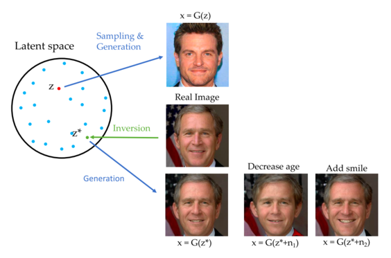
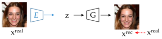
GAN inversion aims to obtain the latent vector for any given image, such that when passed through the generator, it generates an image close to the real image. Obtaining the latent vector provides more flexibility to perform image manipulation on any image instead of being constrained to GAN-generated images obtained from random sampling and generation. Fig. 4 shows an illustration of GAN inversion.
The inversion problem can be defined as:
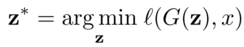
such that z refers to a latent vector, G refers to the generator, l refers to the distance metric in the image space such as l1, l2, perceptual loss, etc., applied at pixel-level.
2.2 GAN inversion approaches
Previous researches have explored three main inversion techniques. The generator has been trained beforehand.
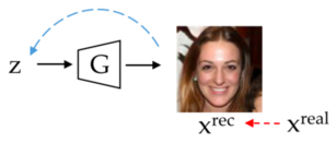
- Optimization-based: optimizes the latent vector z to reconstruct an image xʳᵉᶜ close to the real image x. The objective function is defined as follows:
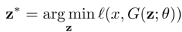
where θ refers to the trained parameters of G.
Various approaches perform optimization using gradient descent. The optimization problem is highly non-convex and requires a good initialization, else risks being stuck in local minima. It is important to note that the optimization procedure is performed during inference and can be computationally expensive, requiring many passes through the generator each time a new image is to be mapped to its latent vector.
- Learning-based: incorporates an encoder module, E, trained using multiple images X generated by G with their corresponding known latent vectors Z. The encoder module aims to generate a latent vector zₙ for the image xₙ , such that when zₙ is passed through G, it reconstructs an image closer to xₙ.
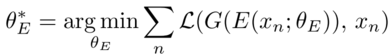
The encoder architecture generally resembles the discriminator D architecture, only differing on the final layers. It generally performs better than a basic optimization approach and does not fall into a local minima. It is worth noting that the latent vector can be obtained directly by passing the image through the encoder during inference.
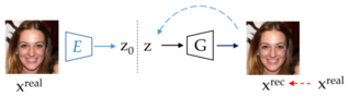
- Hybrid-based: incorporates both the above-mentioned approaches. Similar to learning-based approaches, they train the encoder using images generated by G. During inference, the real image x is passed through E to obtain z, which serves as an initialization for the latent vector for optimization to further reduce the distance between x and xʳᵉᶜ.
3. Differences from VAE-GANs
Variational Autoencoders (VAEs) are another variant of generative models, proposed by Kingma et al. [7]. VAEs aim to train an encoder-decoder architecture to reconstruct images while also using KL-divergence to ensure that the latent distribution is close to an expected Gaussian distribution, with a defined mean and standard deviation.
Variational Autoencoders Generative Adversarial Networks (VAE-GANs) are a combination of VAEs and GANs, proposed by Larsen et al. [8]. Their architecture can be seen in Fig. 8. On incorporating GANs into the architecture, the VAE decoder serves as the generator, and a discriminator tries to differentiate between a generated and real image. While VAEs tend to produce blurry images, combining them with GANs helped them obtain comparable performance as the baseline GAN architectures on image generation tasks.
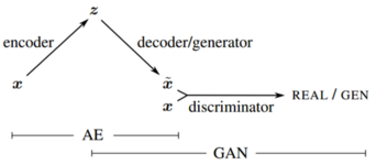
The learning-based GAN inversion architecture constitutes similar modules as VAE-GANs, and this might become a point of confusion. However, these architectures differ in their internal dynamics, their training approach, and their purpose itself.
Learning-based GAN inversion approaches aim to understand the latent space of an already trained GAN as well as obtain a corresponding latent code for an image by training the encoder independently. VAE-GAN, on the other hand, seeks to train the encoder together with the GAN modules to generate images.
4. Summary
In this post, we briefly introduced the concept of GAN inversion and its approaches. In the following parts, we will give a detailed analysis of some GAN inversion researches and focus on its extensions, applications, and latent space navigation with GAN inversion.
Read GAN Inversion: A brief walkthrough — Part II here
References
[7] Kingma, D.P., & Welling, M. (2014). Auto-Encoding Variational Bayes. CoRR, abs/1312.6114.
Written by: Sanjana Jain, AI Researcher, and Sertis Vision Lab Team
Originally published at https://www.sertiscorp.com/