A Practical Time-Series Forecasting Guideline For Machine Learning — Part II

In Part I, we briefly introduced the concept of time series and provided guidelines for assessing forecastability. In this article, we’ll focus on the dos and don’ts of time-series forecasting, providing practical guidelines during the model development phase.
Model Development
Before we delve into model development, let’s establish a fundamental principle:
“Simple but elegant.”
Why prioritize simplicity?
In the experimentation, we might end up accumulating numerous features, employing multiple models, or implementing complex pre-processing steps — all in pursuit of higher accuracy. However, this approach often leads to increased complexity and maintenance challenges.
We advocate starting with simplicity. Begin with straightforward models and processes, and only introduce complexity when necessary to address specific challenges or improve performance. This approach not only facilitates initial development but also ensures sustainability and ease of maintenance as you progress.
Starting with a Baseline Model
Begin by establishing a baseline model — a simple and straightforward approach that can be implemented quickly and easily. The primary objective of a baseline model is to serve as a benchmark for assessing whether more complex models are performing adequately.
The most commonly used baseline models include simple statistical methods or univariate time-series models such as naive window averages, exponential smoothing, or other basic forecasting techniques. These models provide a foundational starting point to evaluate the performance and effectiveness of more advanced modeling approaches
Start Developing the Model
Focus on Feature Engineering
Once you have established a baseline model, the next step is to select the appropriate model and features. You might wonder which model is the most powerful for time series forecasting. Unfortunately, no single model fits all scenarios. Each model has its advantages and disadvantages, which vary depending on the specifics of your data.
We recommend dedicating time to developing sophisticated features rather than focusing solely on finding the perfect algorithm. Effective feature engineering can significantly enhance your model’s performance and provide deeper insights into your time series data.
Understand Feature types
There are three types [1] of features that can help improve the performance of machine learning models for time series forecasting. However, caution is needed when working with each type.
- Past Covariates
Past covariates represent historical information, such as sales from the previous month, temperatures over the last seven days, or rolling sales averages over the past seven days. These historical data points are commonly referred to as “lag” values. You can create lag values using the pandas.DataFrame.shift function in Python.
Tips for Creating Lag Values
You might wonder which lag values to create. Here are some guidelines:
- Create lag values following the seasonality: Identify the seasonality in your data, such as daily, weekly, or monthly patterns. Create lag features that align with these periods. Remember an acf plot mentioned before, we observed hourly seasonality. Thus, we consider creating lag values for 24, 48, and 72 hours prior. This helps the model capture recurring patterns and improve forecast accuracy.
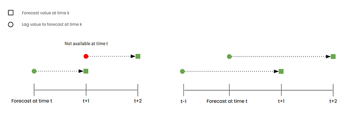
- Ensure time lags are greater than the forecast horizon: The forecast horizon is the number of time steps you aim to predict into the future. When creating lag features, make sure the lag period is greater than your forecast horizon to avoid data leakage. For example, if your forecast horizon is one week, create lag features based on data older than one week. This ensures the model uses only past information for predictions. For instance, we are on Monday and would like to forecast 2 days ahead. We cannot use lag day-1 as a feature since forecasting value on Wednesday requires value on Tuesday which is currently not in our hands.

2. Future Covariates
Future covariates refer to additional information we know in advance, such as promotion schedules or weather forecasts. However, it’s crucial to be aware of potential data leakage issues.
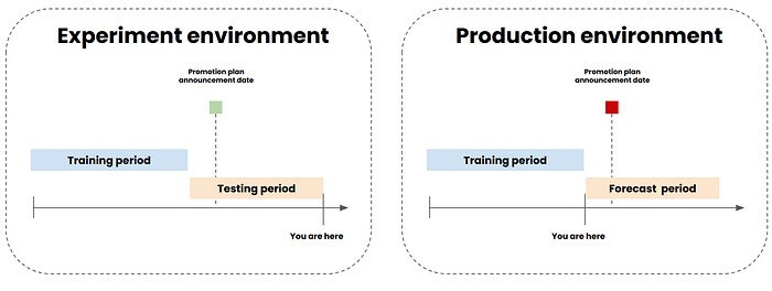
Ensure you know the data before the forecasting period: When conducting experiments and backtesting (splitting historical data into training and testing sets) to evaluate model performance, be cautious not to inadvertently include future information that the model shouldn’t have access to. For example, if you are in May and need to forecast demand for June and July, with a training set from January to March and a test set for April and May, you must ensure that the future covariates used are genuinely known before the forecasting period.
Consider a scenario where your marketing team announces promotions one month in advance. In your experiment, you can use the promotion periods for March and April as features since they were already announced. However, when deploying the model in production, you can’t use future promotion information for July unless it has been announced by June. This ensures your model’s predictions are based on information that would be available in a real-world setting.

3. Static covariates
Static covariates are variables that remain constant over time, such as date, time, and product ID. To utilize these covariates effectively in your model, you need to encode them appropriately. Common encoding techniques include Label Encoding, One-Hot Encoding, and Cyclical Encoding. In time series analysis, Cyclical Encoding is particularly popular. This technique transforms date or time information into sine and cosine waves, capturing the cyclical nature of time series data.
Now, you are successfully creating features without a data leakage problem. In the next part, we will discuss selecting a loss function guideline
Select the right loss function
Since we treat a time series as a regression problem. In regression problems, the default loss function is Mean Squared Error (MSE). However, alternative loss functions can sometimes yield better accuracy depending on use cases. Here are examples of other loss functions:

- Quantile loss: This loss function is useful when you want the model to over-forecast or under-forecast by selecting a specific quantile (q). For q > 0.5, the model penalizes over forecast [⁷].

2. Poisson loss: Poisson loss is typically used for forecasting count data, such as the number of customer arrivals. It assumes that the target variable (Y) follows a Poisson distribution, meaning negative values are not permissible with this loss function [⁷].

Check the model robustness
Once you come up with a set of features, parameters, and models. You certainly do cross-validation to check the model’s robustness. However, You cannot randomly split data as usual since time series data has time time-dependent manner. Temporal splitting data has been introduced to solve this problem. There are 2 temporal techniques expanding window and rolling window [3].

- Expanding Window
In the expanding window approach, the beginning period for each fold remains fixed while the training data increases incrementally with each fold. The test data slides forward for each fold, ensuring that the model is trained on an ever-growing dataset. The expanding window is beneficial for starting with a small data and keeping accumulated data over time.

2. Sliding Window
In the sliding window approach, both the training and test data windows slide forward for each fold. This method maintains a constant window size for training and testing, with both windows moving forward in time together. The rolling window is beneficial for keeping only data and assuming that long-old data may not represent the present or future.

Summary
Congratulations! You now have the knowledge to successfully forecast time series data while avoiding common pitfalls.
Here’s what you’ve learned from Part I & II:
- Time Series Components and Styles: Understanding trends, seasonality, and noise.
- ACF and PACF Plots: Utilizing these tools to identify patterns and select model parameters.
- Tips and Tricks to Avoid Data Leakage: Ensuring data integrity by correctly handling future covariates and creating appropriate lag values.
- Performing Proper Data Splitting: Using expanding and sliding windows for robust cross-validation.
- Selecting the Right Loss Function: Choosing the most suitable loss function for your forecasting needs.
We hope this article helps you execute time-series projects smoothly and effectively.
Reference
[1] Herzen, Julien, Francesco Lässig, Samuele Giuliano Piazzetta, Thomas Neuer, Léo Tafti, Guillaume Raille, Tomas Van Pottelbergh et al. “Darts: User-friendly modern machine learning for time series.” Journal of Machine Learning Research 23, no. 124 (2022): 1–6. Covariates — darts documentation
[2] Terven, Juan, Diana M. Cordova-Esparza, Alfonzo Ramirez-Pedraza, and Edgar A. Chavez-Urbiola. “Loss functions and metrics in deep learning. A review.” arXiv preprint arXiv:2307.02694 (2023). Loss Functions and Metrics in Deep Learning
[3] Hewamalage, Hansika, Klaus Ackermann, and Christoph Bergmeir. “Forecast evaluation for data scientists: common pitfalls and best practices.” Data Mining and Knowledge Discovery 37, no. 2 (2023): 788–832. Forecast Evaluation for Data Scientists: Common Pitfalls and Best Practices
[4] Pedregosa, F. et al., 2011. Scikit-learn: Machine learning in Python. Journal of machine learning research, 12(Oct), pp.2825–2830. 3.1. Cross-validation: evaluating estimator performance
Originally published at https://www.sertiscorp.com/sertis-ai-research
