A Practical Time-Series Forecasting Guideline For Machine Learning — Part I

Introduction
“What quantity of apple juice cartons should we maintain in our inventory?”
“What will be the expected sales volume during the holiday season?”
“Is it possible to forecast electricity consumption to optimize energy production?”
You may have heard these questions before. There are technical difficulties beneath the time-series problem associated with these issues. Time-series forecasting, a fundamental branch of data science, provides a structured approach to tackling these problems by analyzing past patterns to predict future outcomes.
At its core, a time-series problem involves analyzing observations — typically recorded at regular intervals — and using them to make informed predictions. These observations could represent daily sales figures, hourly energy consumption, monthly website traffic data, and so on. The goal is to leverage this historical information to forecast future trends and make strategic decisions.
However, navigating the intricacies of time-series data requires careful consideration of various factors and a data leakage problem (A scenario where you accidentally use future or solution to help model forecast). In this article, we’ll delve into the dos and don’ts of time-series forecasting, providing practical guidelines to help you effectively harness the power of temporal data for actionable insights.
The articles are structured into the following two parts:
- Part I — Introduction to Time-series Data
- Part II — Model Development Guideline
This post is the first part of a two-part series on time-series forecasting guidelines. It aims to briefly introduce the concept of time-series data structure.
Remark: This article will focus on guidelines for treating time series as a regression problem and training a model using tree-based models such as LightGBM, XGBoost, etc only. Statistical models and deep learning frameworks are omitted in this article.
Before You Dive In: Assessing Forecastability
Imagine a typical day at the office as a data scientist — get a new forecasting project requested by business stakeholders. However, before you start experimenting with time-series data, let’s take a moment to assess the forecastability.
Here’s a checklist to help determine forecastability:
Forecast Time Horizon and Granularity
Firstly, define the forecast time horizon — the future time steps you aim to predict. Additionally, consider the granularity of your forecasts, which reflects the time intervals of your predictions. For instance, if you aim to forecast every 15 minutes 24 hours ahead, your granularity would be 15 minutes level and the forecast horizon would be 96(24*4) time steps.
Data Availability
- Checking historical target data, This critical step ensures feasibility between your forecasting horizon and available data. For instance, if tasked with predicting next year’s monthly sales (forecast horizon: 1 year, granularity: monthly level), but you only have six months of historical sales data, achieving accurate results could be challenging.
- Checking the exogenous variable, While time-series data relies on historical patterns for forecasting, incorporating external factors — known as exogenous variables — can significantly boost model performance. For example, having advanced knowledge of promotions can improve sales forecasts. While not mandatory, leveraging exogenous variables is often key to achieving high forecast accuracy.
Assessing these factors upfront can determine the project’s viability and potential for success. It’s essential to ensure that your forecasting goals align with the data at hand, setting realistic expectations and paving the way for effective time-series modeling.
Exploratory Data Analysis (EDA)
EDA is a foundational practice in data science, essential for understanding the behavior and characteristics of data. Time-series data, in particular, exhibits unique patterns that require unique analysis techniques. Let’s begin by exploring the fundamental components of time series data.
Time-Series Components
A single time series can typically be deconstructed into three main components:
Trend
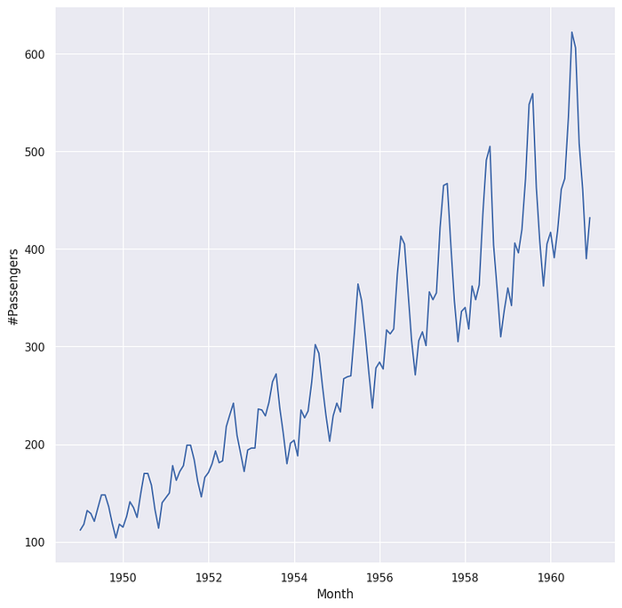
A trend signifies a long-term directional movement in the data, which can be either increasing or decreasing over time. Trends may exhibit nonlinear behavior, transitioning from growth to decline or vice versa. Referencing Figure 1 below, we observe an upward trend in the number of passengers over a 12-year period.
Seasonality
Seasonality manifests as predictable fluctuations within a time series, often influenced by recurring factors such as the time of year or day of the week. Seasonal patterns occur at fixed and identifiable intervals. As depicted in Figure 1 below, strong monthly seasonality is evident in the data.
Noise
Noise represents the stochastic, random variations present in the data. These fluctuations are considered unpredictable and independent of one another. Noise may not be visually apparent in a graph. We will delve deeper into noise and its implications in subsequent discussions.
Time-Series Equation
Time-series data can be mathematically represented using equations that capture the interplay of its fundamental components. There are two primary equation styles commonly used for time series analysis.
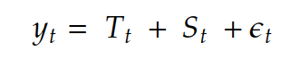
- Additive time-series
The additive time-series equation is expressed as:
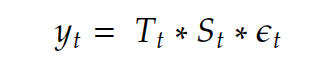
2. Multiplicative time-series
The multiplicative time-series equation is formulated as:
Where
- Y_t represents the observed data at time t
- T_t represents the time-series trend at time t
- S_t represents the seasonality of time-series at time t
- e_t represents the error or noise of data at time t
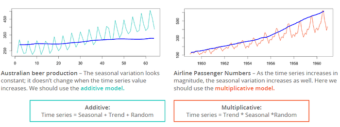
By long story short, the additive model represents a seasonal variation. For the additive model, the magnitude of seasonality doesn’t change when the trend increases/decreases. In contrast, the seasonality magnitude of the multiplicative model changes dramatically when trends go up or down.
These equations provide a structured framework for understanding how trends, seasonal patterns, and random fluctuations interact within time-series data. These equations will play a key role when using time-series models, especially in statistical models.
Time-Series Decomposition
Once you grasp the concept of time-series components and equations, you might be curious about how to effectively decompose these values to extract meaningful insights. Several methods exist for decomposing time series, including SEATS, X-11, naive, and STL methods [2]. All of these methods are available on the statmodel package. The information from time series decomposition is very useful in the model development part.
In this article, we will focus on practical applications of time-series decomposition without delving into the mathematics behind it. For those interested in a deeper dive into the methodology, further details can be found in the associated research paper [2].
Remark: the figure below uses “statsmodels.tsa.seasonal.seasonal_decompose” to decompose. There is a parameter called “model” which allows passing time series type whether “additive” or “multiplicative” [3]. So, knowing the time series type by visual inspection can help us to choose the right parameter.

ACF and PACF
The autocorrelation function (acf) and partial autocorrelation function (pacf) are fundamental statistical tools in time series analysis. Plotting the acf and pacf values can reveal insights into the trend and seasonality within the time series data.
- ACF (auto-correlation function)
acf quantifies a linear relationship between the value at time t and the value at time t+k
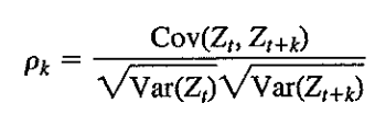
Where
- rho_k represents the correlation between value at t and t+k
- Z_t represents the value at time t
- Z_t+k represents the value at time t+k
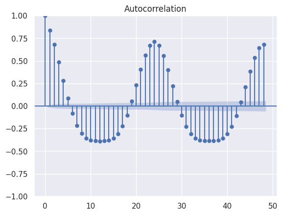
In this plot above, noticeable spikes occur at regular intervals of 24 hours, indicating significant auto-correlation at these lags. This pattern possibly reflects consistent seasons over the days. Moreover, knowing the acf pattern is helpful information for identifying the suitable parameters of the Moving Average model.
2. PACF (partial auto-correlation function)
Since, the auto-correlation may suffer from linear dependency for example, if we know that there is a strong linear relationship between time t and t+1. There might be a strong relationship between t and t +2 too. Since t+1 and t+2 are also a strong relationship. pacf has been introduced to overcome this problem [5].
The pacf value represents the relationship between the value at time t and t+k and removing t+1,t+2, …, t+k-1. The pacf exact calculation formula is omitted in this article but you can see the calculation formula in the link below.
While autocorrelation (acf) can suffer from linear dependencies — for instance, if there’s a strong linear relationship between time t and t+1, which may extend to t+2 due to the relationship between t+1 and t+2 — the partial autocorrelation function (pacf) offers a solution to this issue.
pacf measures the specific relationship between the value at time t and t+k, while removing the influence of intermediate time steps t+1, t+2, …, t+k-1. The exact calculation formula for pacf is not detailed in this article.
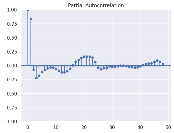
In the plot above, a significant correlation is observed between lag t and t+1. Additionally, pacf plots are instrumental in determining the parameters for constructing an Autoregressive model.
Summary
Now that we have pointed out the forecastability assessment with a given checklist. We also have briefly explained concepts of time series data through exploratory analysis and time-series descriptive statistics.
In the following part, we will explain about developing time-series model guidelines, do, and don’t during experimentation.
[1] Data = Seasonal + Trend + Random: Decomposition Using R
[2] Hyndman, Rob J., and George Athanasopoulos. Forecasting: principles and practice. OTexts, 2018. Forecasting: Principles and Practice (3rd ed)
[3] Seabold, Skipper, and Josef Perktold. “Statsmodels: econometric and statistical modeling with python.” SciPy 7 (2010): statsmodels.tsa.seasonal.seasonal_decompose — statsmodels 0.14.1
[4] WEI, William WS. “Univariate and Multivariate Methods.” TIME SERIES ANALYSIS (2006). (Second Edition)”
Originally published at https://www.sertiscorp.com/sertis-ai-research