Latent Diffusion Models: A Review — Part I

7 min readSep 28, 2023

This series aims to explain the mechanism of Latent Diffusion Models (LDMs) [1], which are a type of latent text-to-image diffusion model. In addition, it also aims to provide a summary of its recent applications. The posts are structured into the following two parts:

Part I — Introduction to Diffusion & LDMs
Part II — Applications of LDMs

This post is the first part of a two-part series on LDMs. It aims to briefly introduce the mechanism of diffusion models and how they connect to variational autoencoders in generating samples matching the original data after a finite time. In addition, this blog-post aims to explain the mechanism of LDMs and how it differs from the standard formulation of diffusion models.

1. What are Diffusion Models?

Over the past decade, deep generative models, such as generative adversarial networks (GANs), auto-regressive models, flows, and variational autoencoders (VAEs), have shown to achieve impressive results in image synthesis [2, 3, 4, 6]. Recently, diffusion probabilistic models (DPMs) [13], a class of of likelihood-based models, have emerged as the new state-of-the-art (SOTA) deep generative models exhibiting competitive performance to other SOTA approaches in various computer vision tasks such as image super-resolution [7], in-painting [1], and semantic segmentation [9]. Being likelihood-based models, DPMs do not exhibit mode-collapse and training instabilities as GANs and, by heavily exploiting parameter sharing, they can model highly complex distributions of natural images with- out involving billions of parameters as in auto-regressive models. Furthermore, DPMs have shown great potential in other research areas such as natural language processing [5], temporal data-modelling [8, 10] and multi-modal learning [11, 12] .

As shown in Figure 1, a DPM consists of two Markov chains — the forward chain, which is hand designed and fixed, systematically perturbs the data distribution, x₀ , by gradually adding Gaussian noise with a pre-designed schedule until the data distribution converges to a given prior xᴛ. On the other hand, the reverse chain samples from this prior distribution and gradually produces less-noisy samples xᴛ₋₁ xᴛ₋₂, … until reaching the final sample x₀. Each time step t corresponds to a certain noise level, and xₜ can be thought of as a mixture of a signal x₀ with some noise ε where the signal to noise ratio is determined by the time step t. Usually a DPM uses a neural network that learns to produce a slightly more “denoised” xₜ₋₁ from xₜ.

**Figure 1.** The data modelling process in DPM (image from [14]). The forward and the reverse chains are denoted by solid and dashed lines respectively.

Given a data distribution x₀~ q(x₀), the forward noising process produces latents x₁, x₂,…, xᴛ, at each time step, by adding Gaussian noise with variance βₜ ∈ (0,1) as :

where q(xₜ) denotes the distribution of latent variable xₜ in the forward process. This process of adding noise is repeated until the distribution of xᴛ is practically indistinguishable from pure Gaussian noise N(xᴛ| 0, I) . Thus, the reverse chain entails estimating a joint distribution pθ(x₀:ᴛ) as :

where p(xᴛ) = N(xᴛ| 0, I) and pθ(xₜ) denotes the estimated distribution of the latent variable xₜ. The estimated joint distribution is learned via optimizing the variational upper bound on the negative log-likelihood as:

The above training objective is equivalent to maximizing the Evidence Lower BOund (ELBO), a lower bound estimate on the log marginal probability density of the data, in VAEs [15]. A DPM can be considered as a hierarchical Markovian VAE with a prefixed encoder. Similar to a VAE encoder, the forward process in a DPM aims to map input data into a continuous latent space at different time steps, while the reverse process aims to recover the original data distribution via optimizing the above training objective, similar to a VAE decoder. As such, optimizing a diffusion model can be viewed as training an infinite, deep, hierarchical VAE.

2. Latent Diffusion Models

DPMs belong to the class of likelihood-based models, whose mode-covering behavior makes them capable to model imperceptible details of the data. Thus, in the case of image synthesis, DPMs typically operate directly in pixel space, and therefore optimizing a high-resolution image generating DPM often consumes hundreds of GPU days and also making inference expensive due to sequential evaluations.

Rombach et al. [1] introduced the concept of LDMs, which aimed to reduce the computational complexity to enable DPM training on limited computational resources while retaining their quality and flexibility. The key idea of LDMs is to separate the training into two phases :

Perceptual image compression: This is the first stage of training in which an autoencoder is trained which provides a lower-dimensional (and thereby efficient) representational space which is perceptually equivalent to the data space.
Latent Diffusion: In this second phase, a DPM is trained on the learned lower-dimensional latent space from the trained autoencoder, instead of the high-dimensional pixel space. In addition to making training scalable, the reduced complexity also provides efficient image generation from the latent space with a single network pass.

2.1 Perceptual Image Compression

For the first stage, Rombach et al. [1] employ an autoencoder training approach that integrates a perceptual loss and a patch-based adversarial objective, thus constraining reconstructions to adhere to the image manifold. This strategy promotes local realism and mitigates the introduction of blurriness often associated with relying exclusively on pixel-space losses like L2 or L1 objectives. Given an image x ∈ Rᴴ×ᵂ×³ in RGB space, the encoder maps x into a latent representation z ∈ Rʰ×ʷ×ᶜ, while the decoder reconstructs the image from its subsequent latent representation. More precisely, the encoder downsamples the image by a factor f = H/h = W/w. This process of transforming a high-dimensional RGB image into a compressed two-dimensional representation allows the DPM to work with this two-dimensional structure of the learned latent space in which high-frequency, imperceptible details are abstracted away. This latent space is more suitable for likelihood-based generative models, as they can now (i) focus on the important, semantic bits of the data and (ii) train in a lower dimensional, computationally much more efficient space. Furthermore, in order to avoid high-variance latent space, Rombach et al. [1] experiment with two different types of regularization: KL-reg [15], similar to a VAE and VQ-reg [18]. Thus, the forward chain in a DPM is already taken into consideration while training the autoencoder as the encoder learns to estimate the distribution of the learned latent space in the process.

In their work, Rombach et al. [1] train the autoencoder on images of size 256x256 from CelebA-HQ [20], FFHQ [21], LSUN-Churches and -Bedrooms [22] datasets.

**Figure 2.** The overall pipeline for LDM as proposed by Rombach et al. [1] (image from [1]).

2.2 Latent Diffusion

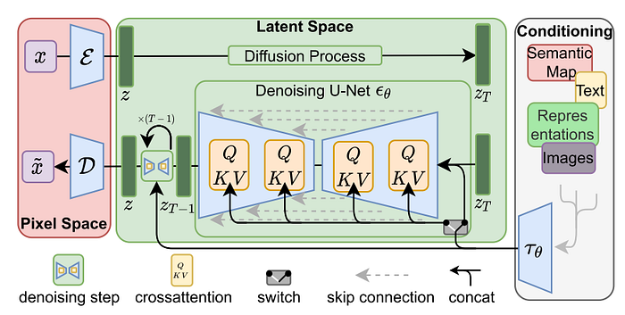
Once the autoencoder is learned the DPM forward chain entails sampling zₜ directly from the encoder during this second stage training. For the reverse process, Rombach et al. [1] use a time-conditional UNet [17]. Additionally, Rombach et al. [1] exploit the capability of DPMs to model conditional distributions. For this purpose, they turn their proposed LDM into a more flexible conditional image generator by augmenting the underlying UNet backbone with the cross-attention mechanism [19] — an effective way for attention-based models to learn various input modalities. Rombach et al. [1] introduce yet another encoder τθ, a transformer, which converts the input from a different modality in the form of text prompts into an intermediate representation that is then mapped to the layers of the UNet via multi-head cross-attention. During this second stage, both the time-conditional UNet and τθ are jointly optimized. The proposed pipeline is illustrated in Figure 2. This combination of language representation and visual synthesis results in a powerful model, which generalizes well to complex, user-defined text prompts as illustrated in Figure 3.

**Figure 3.** Example of text-to-image synthesis using the LDM approach as proposed by Rombach et al. [1] (image from [1]).

3. Summary

We have briefly introduced the concept of DPMs and explained how the forward and the reverse process in a DPM resemble a hierarchical VAE. Additionally, we cover the problem of high computational complexity of traditional DPMs and how the formulation of LDMs has helped address this issue. In the following part, we will cover the key applications of LDMs and how it has paved the way for a specific configuration of its architecture known as Stable Diffusion [16].