Introduction
Computer vision is constantly getting increased attention lately, due to interest in capability of deep learning models [1,2,3]. With these technologies, we can utilise information encoded in images and leverage them to tackle more real-world problems never before imagined to be solved by computers.
One of the most overlooked pieces of information implicitly encoded in images is the depth information which is lost due to the process of 2D image formation. Since images are in 2D, most vision tasks today, which utilise these images, only involve information in 2D. However, since the physical world also contains information about depth, it is much more suitable to use 3D information to tackle real-world problems. Applications which utilises 3D information include 3D facial expression recognition [4], 3D tracking [5, 6, 7], data augmentation [8] and autonomous vehicles [9, 10].
The process of recovering depth information from 2D images is by no means, unfamiliar to us humans. We humans perform this complex process in a blink of an eye all the time. We perceive the physical world in 3-dimensional. But how exactly? The human eyes, each of them only captures 2D information but with slightly different position, the brain then combines their information and calculates the depth information of the perceived real-world scene. This process is thus called 3D reconstruction. Therefore, this means, we should be able to capture 3D information of real-world scenes if we have more than one camera, as is the case with human eyes.
In this article, we’re going to cover some of the fundamental knowledge regarding 3D reconstruction from simple mathematical camera models to the process of depth calculation using stereo cameras.
Basics
Camera models

In order to understand how we can recover depth from 2D images, we need first to understand how real-world scenes in 3D can be captured into 2D images. Such a process can be mathematically explained by camera models.
The simplest of such mathematical models is the “Pinhole camera” model depicted in Figure 1 [11]. In this model of camera, the real-world point X = [x, y, z]ᵀ is projected to image plane p by a ray passing from X to the center of camera C. The intersection point of the line XC and the image plane p is where point X is projected as x = [x, y]ᵀ on the image. f is called the focal length of the camera and is the distance between the camera center and the image plane. Point x can then be mathematically expressed by the following equation:

where P is the camera matrix defined by:

where K is the intrinsic camera matrix expressed by:

Parameters f, pₓ and pᵧ are the focal length, and x, y coordinates of the principal point (normally assumed to be the center of the image) of the camera, respectively. R and t are rotation matrix and translation vector (collectively called extrinsic camera parameters) used to transform real-world coordinates into camera coordinates. Since normally, an object in the real world would be expressed with different coordinate to camera coordinate as in Figure 2. We need to change the coordinate of the object to that of the camera first before we can project it onto an image. This is where extrinsic camera parameters come in, they are defined as:

All these camera parameters an be obtained by a process called camera calibration. It is a process of calculating the camera’s intrinsic variables using a known property of an object being captured, for example, a chess board. Essentially, with all these parameters we can now convert real-world coordinates into the image pixel’s coordinates.

Stereo camera model
In a setting with more than one camera, we are finally able to calculate depth information, which was lost in an image capturing process, hence, 3D reconstruction.
Triangulation
As we can see in the Pinhole camera model, depth information, z, is lost from the projection of point X onto image plane p. In this situation, if we only know point x₁ (say, pixel coordinate of point X projected on image plane p₁), real-world point X, can lie anywhere along the ray XC.
However, in a stereo camera model (see Figure 3), we have two cameras pointing to the same scene. Given that we know points x₁ and x₂ (which are point X projected on the two image planes via rays XC₁ and XC₂), we can find where the rays XC₁ and XC₂ intersect in the 3D space and hence re-calculate the 3D position of X. The process is called triangulation.
The aforementioned is the concept of how should it be done mathematically, in order to actually execute this, there are some more processes required, namely, stereo calibration and point matching.
- Stereo calibration — the process used to find relative position of the second camera with respect to the first camera
- Corresponding point matching — the process of finding corresponding points in one image captured on the other camera.
How to know camera positions relative to one another? Stereo calibration
The previous section explains how to calculate depth using triangulation. However, this assumes we know the position of the second camera with respect to the first one. In practice, this is done through a process called stereo camera calibration. Stereo calibration basically requires the two cameras to capture the same scene with some known property, for example, capturing a chessboard (in this case, known property being that the chessboard is a planar object and each grid has the same length) image with different view at the same time. This process simply calculates what’s called an essential matrix which encodes the transformation from one image plane to another image plane in the stereo camera setting implicitly giving us the position of the other camera with respect to the first one.
How to find corresponding points? Point matching
In order to perform triangulation of any real-world point X, we need to know its coordinates x₁ and x₂ on both images. To do that, we would need a way to match a point on one image with a point on the other, i.e., finding corresponding points. This process called point matching, a common problem in computer vision where we would like to find points or groups of points in multiple images which correspond to the same object. Conventionally, common matching algorithms are used for this purpose such as SIFT [12], SURF [13] or ORB [14].
Relying on point matching is a good start. However, without any constraint on where to look for the corresponding point in the other image, this can lead to performance and efficiency problems. For example, many areas in an image can have similar appearance. To reduce the search space of point matching, we introduce here epipolar geometry.
Epipolar Geometry
To perform triangulation effectively and efficiently, one can leverage the use of a geometry of stereo camera which enforces constrain on corresponding points. Such geometry is called epipolar geometry.

In epipolar geometry, two cameras pointing at the same scene capturing two images as depicted in Figure 3. There are a few additional terminologies shown here.
- Baseline: The line connecting the two epipoles
- Epipolar line: The epipolar line is the 2D image projection of the 3D ray that passes through a 3D point and the optical center of the other camera.
- Epipolar plane: The plane encompassing point X and the camera centers of both camera centers C₁ and C₂. Each real-world point will have its corresponding epipolar plane.
Observing this model, we see that a point in one image can be represented by a line in the other image (projecting ray XC₁ onto camera C₁ creates the dotted line) and vice versa. We call these lines epipolar lines (illustrated in Figure 3 as e₁ and e₂). Now, let’s say we want to find the corresponding point of point x₁ on the right image (i.e., x₂), the search space can be significantly reduced using epipolar geometry. First, we know that point x₁ lies on ray XC₁ and second, epipolar line e₂ is the projection of ray XC₁ on the right image. Therefore, we only need to look for the corresponding point x₂ along epipolar line e₂ in the right image.
Special case of epipolar geometry
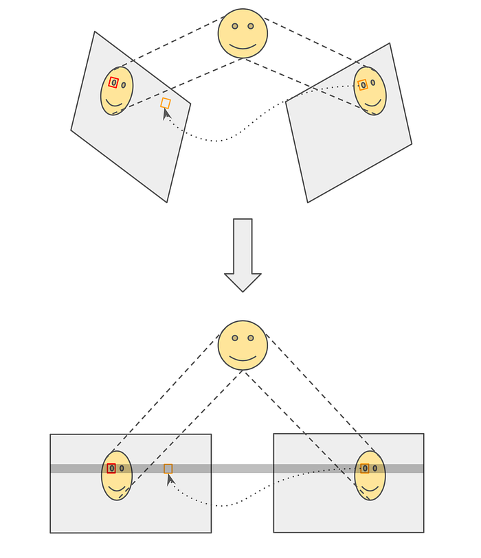
We can further make this point matching search space even smaller by what is called a stereo rectification. The process only needs the parameters of both cameras and the essential matrix obtained in stereo calibration. Recall in Figure 3, epipolar geometry only assumes two cameras point at the same object, however, it does not require the image plane to be parallel. It appears, apparently, parallel image planes have an interesting property. Take a look at Figure 4, in the top is the normal stereo camera setting, corresponding points can differ in both horizontal and vertical axes. In contrast, in the bottom model, image planes are placed in parallel and in this case, corresponding points only differ in their horizontal axis, i.e., epipolar lines are horizontal. This simplifies the search for corresponding points even more and can lead to improvement in both the effectiveness and efficiency of stereo point matching algorithms.

Stereo disparity
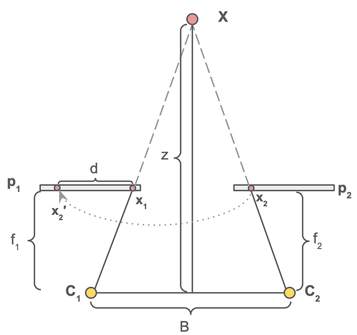
Stereo disparity is the way to calculate the depth of 3D points using two corresponding points. Imagine looking at a scene with one eye and constantly alternating between the two eyes. You will see objects constantly moving left and right, this is called disparity. The more the object moves, i.e., the more disparity, when you switch an eye, the closer the object is. Basically, this means disparity is inversely proportional to distance. Now, we can leverage the property of a similar triangle to calculate depth. The depth calculation with a stereo camera is illustrated in Figure 5. What we need in this equation is the distance between the two corresponding points d and the focal length of both cameras, f₁ and f₂, which should be done via camera calibration in advance. The depth can then be calculated using the following equation:


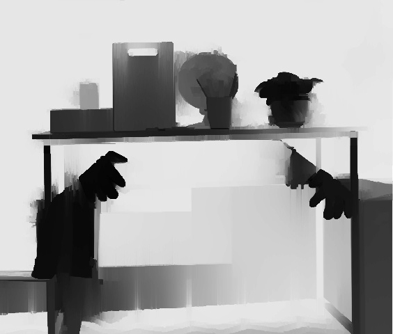
Now that we know how to calculate the depth given a stereo image pair in theory, let’s have a look at an actual result. Figure 6 shows a stereo image pair used in this example. Note that in this case both single and stereo camera calibration are done in advance. We can see the two images are captured at a slightly different angle (the carton on the bottom right of the left image is only partially visible). Using the process aforementioned, we can find the disparity map and use it to calculate the depth of objects in the scene as shown in Figure 7.


No discussion on computer vision would be complete without addressing the transformative impact of deep learning. In Part 2 of this series, we will delve into both traditional approaches and advanced deep learning solutions. Stay tuned for a deeper exploration!
Reference
[1] Kirillov, Alexander, et al. “Segment anything.” Proceedings of the IEEE/CVF International Conference on Computer Vision, 2023.
[2] Radford, Alec, et al. “Learning transferable visual models from natural language supervision.” International conference on machine learning. PMLR, 2021.
[3] Cheng, Tianheng, et al. “Yolo-world: Real-time open-vocabulary object detection.” Proceedings of the IEEE/CVF Conference on Computer Vision and Pattern Recognition, 2024.
[4] Ly, Son Thai, et al. “Multimodal 2D and 3D for In-The-Wild Facial Expression Recognition.” CVPR workshops, 2019.
[5] Ishaq, Ayesha, et al. “Open3DTrack: Towards Open-Vocabulary 3D Multi-Object Tracking.” arXiv preprint arXiv:2410.01678, 2024.
[6] Wang, Siyang, et al. “MCTrack: A Unified 3D Multi-Object Tracking Framework for Autonomous Driving.” arXiv preprint arXiv:2409.16149, 2024.
[7] Meyer, Lukas, et al. “FruitNeRF: A Unified Neural Radiance Field based Fruit Counting Framework.” arXiv preprint arXiv:2408.06190, 2024.
[8] He, Mingjie, et al. “Enhancing face recognition with self-supervised 3d reconstruction.” Proceedings of the IEEE/CVF Conference on Computer Vision and Pattern Recognition, 2022.
[9] Tonderski, Adam, et al. “Neurad: Neural rendering for autonomous driving.” Proceedings of the IEEE/CVF Conference on Computer Vision and Pattern Recognition, 2024.
[10] Khan, Mustafa, et al. “Autosplat: Constrained gaussian splatting for autonomous driving scene reconstruction.” arXiv preprint arXiv:2407.02598, 2024.
[11] Hartley, Richard, and Andrew Zisserman. “Multiple view geometry in computer vision.” Cambridge university press, 2003.
[12] Lowe, David G. “Distinctive image features from scale-invariant keypoints.” International journal of computer vision 60: 91–110, 2004.
[13] Bay, Herbert, et al. “Speeded-up robust features (SURF).” Computer vision and image understanding 110.3: 346–359, 2008.
[14] Rublee, Ethan, et al. “ORB: An efficient alternative to SIFT or SURF.” 2011 International conference on computer vision. IEEE, 2011.
Originally published at https://www.sertiscorp.com/sertis-ai-research
