Graph Neural Networks, Part I: Introduction

9 min readJul 29, 2022

This series of posts aims to talk about the concept and applications of graph neural networks (GNNs), which is a machine learning model applied to graph-structured data. The series consists of three parts as follows:

Part I, which is this part, explains what graph-structured data is and how it is represented. This part also introduces the concept of graph machine learning and GNNs.
Part II provides more details on a variant of GNNs called graph convolutional networks (GCNs). Two main types of GCNs, i.e., spectral GCNs and spatial GCNs, are explained.
Part III describes various applications of GNNs to real-world problems, for example, visual question answering, molecular property prediction, recommendation systems, traffic forecasting, and so on.

1. What is a graph?

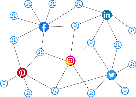
A graph is a data structure representing a collection of entities as nodes and their relations as edges. It is used to model pairwise relations between objects. The connectivity information or pairwise interaction between entities represented in graphs provides additional information about the relationship between the objects. For example, a user in a social network has different attributes such as name, age, gender, contacts, etc. These attributes do not give any information on how one user is connected to another (Fig. 1). We could use an unsupervised clustering method to form sets based on users’ locality, age, etc., and hypothesize their social or work relations. However, without explicit modeling of their interactions, it is hard to get any useful information. Graphs can represent such interactions where the nodes represent the users, while social interactions, such as friendship, colleagueship, or being family relatives, are modeled by the connectivity information between nodes. Another example of data that can be represented by a graph is a chemical compound in which the atoms are represented as nodes and the chemical bonds connecting the atoms are represented as edges (Fig. 2).

Fig. 1: A social graph in which nodes represent the users and the edges represent the connection

**Fig. 2:** A hydrocarbon molecule, ethanol, is represented as a graph in which the individual atoms are represented as nodes and the chemical bonds between atoms are represented as edges.

How do we define a graph?

A graph can be denoted as G = {V, E }, where V = {v₁, v₂, …, vₙ} is a set of n = |V | nodes and E = {e₁, e₂, …, eₘ} is a set of m = |E | edges. The order of a graph is determined by its number of nodes, n, and the size is defined by its number of edges, m. If two arbitrary nodes vᵢ and vⱼ are connected via an edge eₖ, it can also be represented as eₖ = (vᵢ, vⱼ ). A graph can be directed or undirected. In a directed graph, an edge has a direction associated with it whereas, in an undirected graph, the order of two nodes does not matter. A node vᵢ is adjacent to another node vⱼ if and only if there is an edge connecting them.

How do we store graph data?

A graph can also be represented as an adjacency matrix, which describes the connectivity between the nodes (Fig. 3(b)). The adjacency matrix is denoted as A ϵ {0, 1}ⁿˣⁿ. The (i, j) entry of the matrix, denoted as Aᵢ,ⱼ, represents the connectivity between the two nodes vᵢ and vⱼ, i.e. Aᵢ,ⱼ = 1 if vᵢ is adjacent to vⱼ; otherwise Aᵢ,ⱼ = 0. For an undirected graph, its corresponding adjacency matrix is symmetric, i.e., Aᵢ,ⱼ = Aⱼ,ᵢ. For a weighted graph, the entry at Aᵢ,ⱼ represents the weight associated with the edge between nodes i and j.

The adjacency matrix formulation of graphs addresses the complex problem of representing graph connectivity. However, this representation has some drawbacks. Graphs in the real world can be very large, e.g., containing millions of nodes, and their edges are highly variable. For example, a social graph can have millions of nodes but there are not many edges since connections between users are usually local. Thus, its adjacency matrix can be very sparse and space-inefficient. Another issue with the adjacency matrix is the representation is not permutation invariant, so different adjacency matrices may encode the same connectivity of a graph. In other words, changing the node ordering results in different adjacency matrices although they represent the same connectivity information [1].

A more memory-efficient way is to represent a graph as an adjacency list that describes the connectivity of an edge eₖ between nodes vᵢ and vⱼ as a tuple (i, j) in the k-th entry of the adjacency list (Fig. 3(c)). Since the expected number of edges is much lower than n², it requires much less space than the adjacency matrix to store a graph.

**Fig. 3(a):** A graph with a specific node ordering **Fig. 3(b):** The adjacency matrix of the graph in Fig. 3(a). **Fig. 3(c):** The adjacency list of the graph in Fig. 3(a).

What are the tools used to store and manipulate graphs?

Real-world graph data are generally stored and manipulated using graph databases. They are intended to hold data without constricting to a predefined model. Using graph databases allows relationship query performance to stay constant with increasing graph size. Please refer to [2] for more details. Neo4j [2] and TigerGraph [3] are such graph database applications widely used in industry for graph manipulation.

Where do we use graphs in the real-world?

Graph theoretical ideas are highly utilized by researchers, especially in the areas of network topologies. Various concepts like paths, walks, and circuits in graph theory are used in various applications, for example, the traveling salesman problem, database design concepts, and resource networking.

Graph models are successfully applied in proteomics (the study of proteins) and in the study of metabolic networks. Protein-protein interaction networks are commonly represented in a graph format, in which proteins are represented as nodes and edges correspond to their interactions.

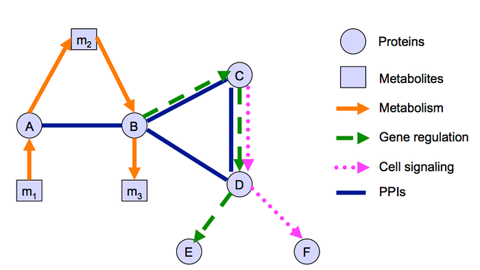
**Fig. 4:** An example of biological interactions represented as a graph. (image from [4])

A real-world application of graphs is a biological network which is a network of biochemical reactions, containing various objects and their relationships. Graphs can model these complex events with molecules, cells, or living organisms as constituents. Nodes in biological networks represent bio-molecules such as genes, proteins, or metabolites, while edges connecting these nodes indicate functional, physical, or chemical interactions between the corresponding bio-molecules (Fig. 4). Please refer to [5] to know more about the applications of graphs in various fields.

2. Machine learning on graphs

The field of research on graph analysis with machine learning algorithms, i.e., graph machine learning, is receiving more attention in recent years because of the expressive power of graphs. Graphs are unique non-Euclidean space data structures. With machine learning techniques, graph data can be used for node classification, link prediction, clustering, etc. Since a graph does not have a natural ordering of nodes, standard neural networks such as multi-layer perceptrons, convolutional neural networks, and recurrent neural networks, in which the features of the nodes are stacked in a specific order, cannot handle the graph input properly. Also, these standard neural networks may use the edge information as additional features of the node but the connectivity is ignored. Graph neural networks (GNNs) are proposed to collectively aggregate information from graph-structured data and model inputs/outputs consisting of elements and their dependency.

Where do we use graph machine learning?

Graph machine learning is used to solve prediction problems on different levels of graphs, namely node, edge, and graph levels. The objective of a node-level task is to predict the property of each node in the graph. For example, predicting which social group a new member would join given their friendship relation and friends’ membership info (Fig. 5). An edge-level task aims to predict whether there exists a relation between two nodes. For example, to predict whether two persons will be the right match for each other. A graph-level task intends to predict a single property of a whole graph. For example, to predict the odor of a newly synthesized chemical compound.

3. What is a graph neural network (GNN)?

The concept of GNNs was first proposed by Gori et al. [6], Scarselli et al. [7], and Scareselli et al. [8]. The task of a GNN is to learn a state embedding that encodes the information of each node and its neighborhood on a graph input. Mathematically, the embedding function f can be defined as:

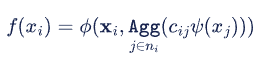
where i is the index of a node being processed; xᵢ is the original node representation of the node i ; 𝜓 is a transformation function applied to its neighbors xⱼ ; c ᵢⱼ is a weight between nodes i and j ; Agg is an aggregator function, such as mean or sum, that fuses neighborhood information; and finally, 𝜙 is a trainable function that transforms the fused information of the node and its neighbors. In summary, we update the node representation by aggregating the node information from the neighboring nodes j using learnable parameters.

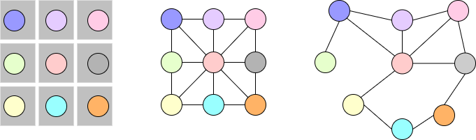
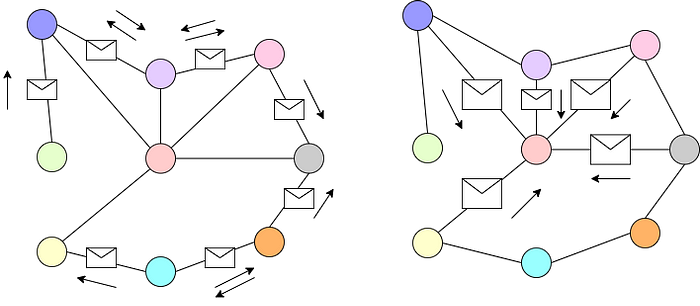
**Fig. 6:** Graph is relaxation of fixed structure and in non-euclidean space.

As shown in Fig. 6, graphs can be considered a relaxation of a fixed structure. In convolution neural networks, we apply a set of learnable filters that aggregates the neighborhood information on a fixed structure such as images. Similarly, we can apply GNNs to both fixed and relaxed structures that are not bounded by Euclidean geometry. We can also think of GNNs as message passing between different nodes aggregating the neighborhood information as shown in Fig. 7.

**Fig. 7:** Messages from nodes two hopes away are accumulated and then passed on to the central node.

Intuitively, the operation performed by GNNs on node representation can be thought of as transforming the embedding space of the nodes into a new space using the gradients of the tasks. The new representation for nodes has all the necessary information about itself and its neighbors related to the task it is being trained on.

4. Summary

We have introduced graph data, its representations, and examples of graph data. We have explained how machine learning is applied to graph data and finally introduced the concept of GNNs, which is the key topic of this series. In the second part, a variant of GNNs called graph convolutional networks (GCN) is described in detail. Two types of GCNs, i.e., 1) spectral GCNs and 2) spatial GCNs, are also discussed.