This blog post is a summary of the peer-reviewed research article Amortized Variational Inference: A Systematic Review, in affiliation with Sertis Vision Lab, published in the Journal of Artificial Intelligence Research (JAIR)
Introduction
Efficient computation of complex probability distributions has been one of the core problems in modern statistics. Solving this problem is of grave importance in Bayesian statistics as its core principle is to frame inference about unknown variables as a calculation involving a posterior probability distribution. Exact inference, which typically involves analytically computing the exact value of the posterior probability distribution over the variables of interest, offers a solution to this inference problem. Algorithms in this category include the elimination algorithm, the sum-product algorithm, and the junction tree algorithm. However, for highly complex probability densities and large data sets, exact inference algorithms favor accuracy at the cost of speed. Additionally, for highly complex probability distributions, exact inference does not guarantee a closed-form solution. In fact, the exact computation of conditional probabilities in belief networks is NP-hard.
As an alternative approach, approximate inference, which has been in development since the early 1950s, offers an efficient solution to Bayesian inference by providing simpler estimates of complex probability densities. Various Markov Chain Monte Carlo (MCMC) techniques, such as Metropolis-Hastings and Gibbs’ Sampling, fall under this category of algorithms. However, MCMC methods that rely on sampling are slow to converge and do not scale efficiently.
Another approximate inference technique, namely Variational Inference (VI), tackles the problem of inefficient approximate inference by the use of a suitable measure to select a tractable approximation to the posterior probability density. The methodology of VI is, thus, to re-frame the statistical inference problem into an optimization problem giving us the speed benefits of maximum a posteriori (MAP) estimation. This makes VI an ideal choice for applications in areas like statistical physics, generative modeling, and neural networks.
Variational Inference (VI)

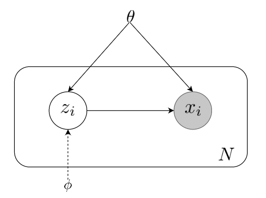
The core principle of VI is to convert the statistical inference problem of computing complex posterior probability densities into a tractable optimization problem. As an approximate inference technique, VI offers an approximation to the true posterior distribution by using a suitable measure. Usually, this measure is chosen to be the non-negative Kullback–Leibler (KL) divergence, which estimates the relative entropy between two densities. In the case of traditional VI, the optimization problem entails reducing the relative entropy by choosing an approximate density with the lowest reverse KL-divergence to the true posterior density, sampling one data point at a time. For each data point, an approximate density, with its own set of parameters (as shown in Figure 1), is selected from a family of tractable densities. The complexity and the accuracy of the VI optimization process are controlled by the choice of this variational family.
Additionally, VI enables an efficient computation of a lower bound to the observed data distribution. This lower bound is popularly referred to as the Evidence Lower BOund (ELBO). The idea is that a higher marginal likelihood is indicative of a better fit to the observed data by the chosen statistical model.
Challenges with traditional VI
The traditional VI optimization problem maximizes the ELBO with respect to the variational parameters for each data point, making this repetitive process introduce a new set of variational parameters for every observation. As a result, the set of optimizable parameters tends to grow, at least, linearly with the observations. Additionally, the VI optimization process is memoryless, i.e., each observation is processed independently of others. This guarantees that inference using one observation will not interfere with another; however, it implies that there is no mechanism to re-use the knowledge from previous observations on newer ones. Thus, inferring on the same observation twice requires the same amount of computation, which is equivalent to inferring on two different ones. When the number of observations is large, it can also lead to extensive computational inefficiency since there is no memory trace of inferences from previous data points.
Amortized VI
“Amortizing” the VI optimization process solves the aforementioned scalability issues as it facilitates keeping a memory trace of inferences from past observations. Instead of optimizing for each data point independently, amortized VI aids in spreading out the optimization cost across multiple data points at a time, reducing the overall computational burden. Therefore, amortized VI makes use of a stochastic function, that creates a mapping between the observed and the latent variables, the latter of which is a sample to the variational posterior distribution whose parameters are learned during the optimization process. Thus, instead of having separate parameters for each observation, the estimated function can infer latent variables even for new data points without re-running the optimization process all over again. This process allows for computational efficiency and flexible memoized re-use of relevant information from past inferences on previously unseen data.
With recent advancements in deep learning, neural networks have been extensively used in the form of the stochastic function for create a mapping between observed and latent variables as well as to estimate the parameters of the posterior probability density. As powerful frameworks, neural networks allow for efficient amortization of inference and have been proven to be a popular choice for efficient scaling to large datasets. Furthermore, the development of GPU-assisted neural network training has also led to the usage of complex neural network architectures with amortized VI, allowing extraction of information from high-dimensional data without human supervision. The variational auto-encoder (VAE) and its variants are primary examples in this case.
Acknowledgements
AI researchers from Sertis Vision Lab, namely Ankush Ganguly, Sanjana Jain, and Ukrit Watchareeruetai co-authored the research paper Amortized Variational Inference: A Systematic Review with the aim to provide an intuitive explanation of the different VI techniques and their applications to researchers new to the field. In addition, the paper is dedicated towards gaining a deeper understanding of the concept of amortized VI while distinguishing it from several other forms of VI. Furthermore, the paper covers how the recent developments in the field of amortized VI have managed to address its weaknesses.
Read our peer-reviewed research here: Amortized Variational Inference: A Systematic Review